Knowing what the model doesn’t know
A neural network answers every question with the same confident voice — inside its training distribution and far outside it. Bayesian methods replace the single answer with a distribution over answers, so the model can finally say the most useful thing a model can say: I’m not sure.
Everything on this page is live. Scan, dig, drag, click — the theory comes after you’ve felt it.You were running Bayes’ rule
Every scan, the game did the same silent move. It weighted each spot’s current believability by how well that spot explains what the detector said. Then it rescaled the bars to sum to one. Here is that single move, frozen mid-update:
Coins wash up near the water
The waterline is at the left end of the beach, so before any scan your belief already leans left. A starting belief can lean — that’s allowed.
BEEP at spot 3
Each bar: how well that spot explains the beep. “It’s under spot 3” explains it well (0.75). Any other spot means it was a false beep (0.25).
Multiply, spot by spot
Left lean × one beep: spot 3 towers, its waterline neighbors keep a little belief, the far end fades. The faint outline is where you started.
Now the vocabulary, attached to things you’ve already touched. The belief bars before the scan are the prior. Each spot’s evidence score is the likelihood. The re-weighted bars afterward are the posterior. In symbols — the one equation this whole note runs on:
On the beach, a beep multiplies the scanned spot’s bar by 0.75 and every other spot’s by 0.25 — silence does the reverse. That’s the whole likelihood. Nothing else happens. That is the algorithm, and it’s the same one running inside any robot that localizes with noisy sensors. The spread of the surviving bars is your uncertainty, measured rather than felt.
Teaching CLIP to say “I’m not sure”
That one move scales all the way up. BayesVLM applies it to vision-language models like CLIP, which score an image–text pair with a single deterministic number — the cosine similarity of their embeddings. That number is just as confident on a distribution-shifted input as on a training-like one: a treasure hunter who digs on the very first beep, at a billion-parameter scale. The recipe (each step is unpacked by the experiments below):
- STEP 1Laplace where it countsKeep the pretrained weights, and fit a cheap Gaussian stand-in for the posterior (the Laplace approximation) over just the last projection layers of the image and text encoders. No training is repeated — Experiment 03 shows why the stand-in earns its place.
- STEP 2Embeddings become GaussiansWith uncertain projection weights, each embedding stops being a point and becomes an (approximately) Gaussian cloud in the joint space: . Familiar inputs give tight clouds. Shifted inputs give diffuse ones.
- STEP 3Uncertainty flows into the scoreThe similarity of two Gaussian clouds is itself a distribution. BayesVLM’s ProbCosine propagates it analytically by moment matching — a mean and a variance for every image–text score, with no Monte Carlo sampling at inference time.
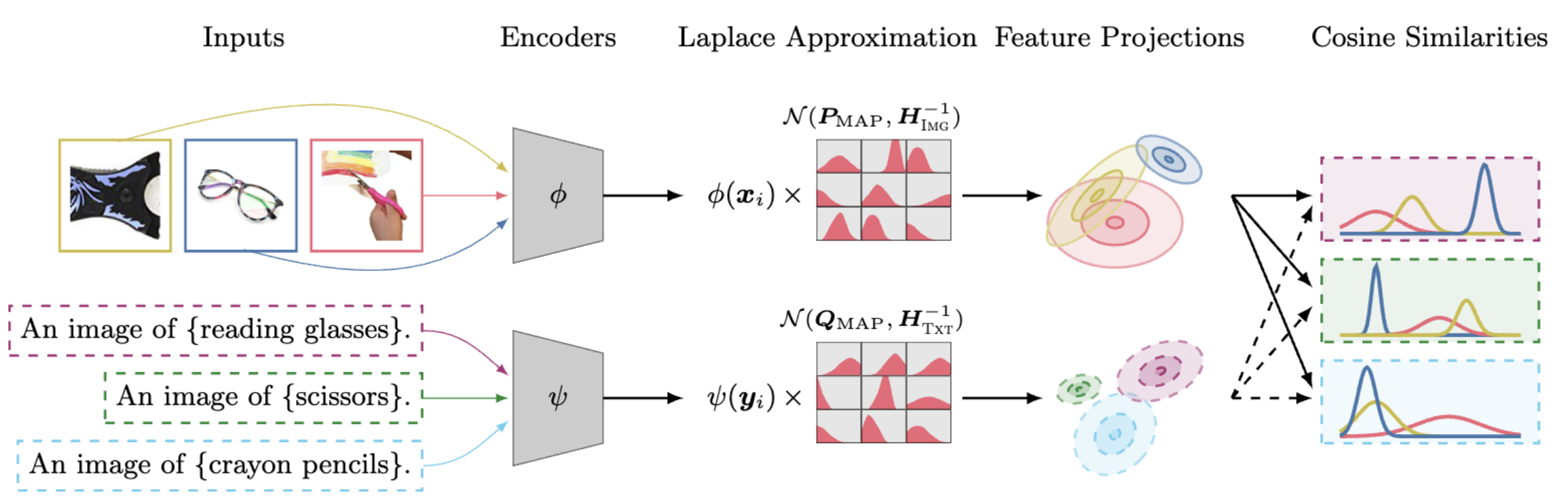
The result: predictions keep the same accuracy but become calibrated — stated confidence finally tracks empirical correctness. And the variance itself is a usable signal. High-variance inputs are exactly the ones worth sending to a human, or worth labeling next (uncertainty-guided active learning). The model didn’t get smarter. It got honest, which in deployed systems is often worth more.
The rest of this note unpacks the two ideas that recipe leans on: what model uncertainty looks like when the candidates are infinite, and why a Gaussian stand-in for a posterior is an honest cheat.
Don’t pick a winner. Keep every candidate.
The beach had nine spots. A regression has infinitely many candidates: every line you could draw through the data is one, and the same rule re-weights them all. The next experiment shows that directly. Gray lines are surviving candidates. Where they disagree, the model tells you it doesn’t know — the “diffuse cloud” from Step 2, in miniature. Try to break it: click two points directly above each other and see what no line can fix.
The integral nobody can do
What you just saw has a formula too. To predict at a new input , ask every surviving candidate and average their answers, weighted by belief — the posterior predictive:
Exact Bayes doesn’t scale
Nine beach spots: trivial. Lines: still closed-form. But a neural network has millions of weights. The candidate space becomes too vast to enumerate, and the integral above becomes hopeless. Every practical method is a different way of cheating. Ensembles train a few networks and treat them as candidates. MC dropout randomizes at test time. Variational inference fits a tractable stand-in by optimization.
Laplace: a Gaussian at the peak
The oldest cheat is the most elegant — and it is the one BayesVLM uses. Training already finds the most believable weights . Taylor-expand the log-posterior there — the linear term vanishes at a maximum — and what is left is a quadratic, which is exactly a Gaussian:
The Hessian measures curvature. A sharp peak means the data pins the weights down (small variance). A flat one means many settings work equally well (large variance). Crucially, this is post-hoc — no retraining, just one curvature computation around weights you already have.
When is the cheat honest?
A Gaussian is symmetric. Real posteriors often aren’t. But posteriors sharpen and symmetrize as data accumulates. The Bernstein–von Mises theorem makes this precise. The experiment below lets you watch the approximation prove itself.
The width is the signal
One move, three scales: belief bars over a beach, a fan of lines over a dataset, Gaussian clouds over CLIP’s embedding space. In every case the answer comes with its own width — and the width, not the answer, is what tells a system when to dig, when to keep scanning, and when to stop and ask for help. For a robot acting in the physical world, that call is the one that matters. Honest beats smart more often than we like to admit.
Further reading: Post-hoc Probabilistic Vision-Language Models (BayesVLM) · Laplace Redux — effortless Bayesian deep learning · Neal, Bayesian Learning for Neural Networks